Fit to Marcenko Pastur Distribution
This post will describe how to use the Marcenko Pastur Distribution (MPD) as a template to identify the presence of signal within a data set.
Practical use:
We will use the MPD distribution as a template to compare the eigen value signature of our data set, against the eigen value signature of random noise. We can obtain a value that quantifies this, and can identify which of the eigen values correspond to the departure from random noise. Identifying this helps us to then target amplification of the signal, or suppression of the noise. In the chart above, 68% of the variance in the data set corresponds to random noise, and eigen values above 1.1 correspond to signal. Applications extend to cybersecurity, credit card fraud, or any other application where you are trying to identify a spurious pattern.
Compute using Python:
# FIle: Fit-to-MPT.py
import numpy as np,pandas as pd
import matplotlib.pyplot as plt
#---------------------------------------------------
def mpPDF(var,q,pts):
# Marcenko-Pastur pdf
# q=T/N
    eMin,eMax=var*(1-(1./q)**.5)**2,var*(1+(1./q)**.5)**2
    eVal=np.linspace(eMin,eMax,pts)
    pdf=q/(2*np.pi*var*eVal)*((eMax-eVal)*(eVal-eMin))**.5
    pdf=pd.Series(pdf,index=eVal)
    return pdf

from sklearn.neighbors.kde import KernelDensity
#---------------------------------------------------
def getPCA(matrix):
    # Get eVal,eVec from a Hermitian matrix
    eVal,eVec=np.linalg.eigh(matrix)
    indices=eVal.argsort()[::-1] # arguments for sorting eVal desc
    eVal,eVec=eVal[indices],eVec[:,indices]
    eVal=np.diagflat(eVal)
    return eVal,eVec
#---------------------------------------------------
def fitKDE(obs,bWidth=.25,kernel='gaussian',x=None):
    # Fit kernel to a series of obs, and derive the prob of obs
    # x is the array of values on which the fit KDE will be evaluated
    if len(obs.shape)==1:obs=obs.reshape(-1,1)
    kde=KernelDensity(kernel=kernel,bandwidth=bWidth).fit(obs)
    if x is None:x=np.unique(obs).reshape(-1,1)
    if len(x.shape)==1:x=x.reshape(-1,1)
    logProb=kde.score_samples(x) # log(density)
    pdf=pd.Series(np.exp(logProb),index=x.flatten())
    return pdf

# Determine matrix with some signal
def getRndCov(nCols,nFacts):
    w=np.random.normal(size=(nCols,nFacts)) # We start with a fully random matrix
    cov=np.dot(w,w.T) # random cov matrix, however not full rank # We calculate the covariance matrix of this fully random matrix
    cov+=np.diag(np.random.uniform(size=nCols)) # full rank cov # We add some constant terms to the above fully random matrix, to represent some signal
    return cov
#---------------------------------------------------
def cov2corr(cov):
    # Derive the correlation matrix from a covariance matrix
    std=np.sqrt(np.diag(cov)) # Determine standard deviation as square root of diagnonal terms (variances)
    corr=cov/np.outer(std,std) # Dividing covariance by product of standard deviations will give you correlation matrix
    corr[corr<-1],corr[corr>1]=-1,1 # numerical error
    return corr
#---------------------------------------------------
alpha,nCols,nFact,q=.995,1000,100,10
cov=np.cov(np.random.normal(size=(nCols*q,nCols)),rowvar=0) # Generate a random matrix and calculate its covariance matrix
cov=alpha*cov+(1-alpha)*getRndCov(nCols,nFact) # noise+signal # Add this random matrix to a matrix containing some signal, with mixing ratio alpha
corr0=cov2corr(cov) # Generate Correlation matrix from Covariance matrix so we can apply Marcenko Pastur Theorem
eVal0,eVec0=getPCA(corr0) # Determine Eigen Values & Eigen Vectors of the Correlation matrix

from scipy.optimize import minimize  # Importing the required optimizers
#---------------------------------------------------
def errPDFs(var,eVal,q,bWidth,pts=1000): # This is the objective function we will minimise
    # Fit error
    pdf0=mpPDF(var[0],q,pts) # theoretical pdf. For each test variance, the optimiser passes, the PDF for that variance, will be calculated using Marcenko Pastur Theorem (MPT)
    pdf1=fitKDE(eVal,bWidth,x=pdf0.index.values) # empirical pdf. The actual data distribution calculated using the Gaussian KDE
    sse=np.sum((pdf1-pdf0)**2) # Calculate difference between ideal random distribution, and actual data distribution. Evaluation is only conducted within range spanned PDF from MPT
    return sse
#---------------------------------------------------
def findMaxEval(eVal,q,bWidth):
    # Find max random eVal by fitting Marcenko’s distp
    out=minimize(lambda *x:errPDFs(*x),.5,args=(eVal,q,bWidth),bounds=((1E-5,1-1E-5),)) # The minimiser is optimising the function errPDF (its objective function) by Varying variance between bounds with .5 as initial estimate
    # .. contd The other parameters required by the objective function are passed separately but remain constant, and are not varied within the optimiser
    if out['success']:var=out['x'][0] # If the optimiser converges, there is an in-built flag called success, which is queried, and the minima is obtained
    else:var=1
    eMax=var*(1+(1./q)**.5)**2 # For the minima variance, calculate the maximum eigen value as per MPT
    return eMax,var
#---------------------------------------------------
eMax0,var0=findMaxEval(np.diag(eVal0),q,bWidth=.01) # Calculate var0 (degree of randomness in actual data), and max eigen value explained by randomness, eigen values above this are due to signal
nFacts0=eVal0.shape[0]-np.diag(eVal0)[::-1].searchsorted(eMax0) # identifying the number of eigen values that contain signal

print(eVal0.shape, eMax0,var0,nFacts0)
pdf1 = fitKDE(np.diag(eVal0), bWidth=.01)  # empirical pdf. The actual data distribution calculated using the Gaussian KDE
plt.plot(pdf1)
plt.show()


Comments
Post a Comment