1.2 Structured Data: Information Driven Bars

This post will describe how to process & store High Frequency financial data to support your Machine Learning Algorithm, based on how much information is contained in the data

The post is directly based on content from the book "Advances in Financial Machine Learning" from Marcos Lopez de Prado

Physical meaning:

This approach is inspired by Claude Shannon's Information Theory, that is the basis of most compression algorithms. Shannon argued that only departure from the norm is new information. A famous example, is that the sun has risen in the morning. Yes, the event has happened, but because the probability of this event was 1.0, this event does not represent information.

In information driven bars, we attempt to use the same insight, to compress the financial data. Here, we know that financial data is inherently noisy, and put guardrails around what level of variance we expect for a particular behavior. It is only when the variance exceeds these guardrails, that we start sampling, as this represents new information. In this way, instead of de-facto sampling every 2000 ticks, we might sample one time for the first 1900 ticks, and ten times for the next 100 ticks, because the data was very volatile in the last 100 ticks. This technique smartly rations your data samples to when you need finer discrimination. 

The end goal remains the same, how do you faithfully capture as much as what happened, with as little data storage used as possible.

Tick run bars: A run is defined as a consistent movement in price, either in the upward or downward direction. This algorithm has a base expectation of how many consecutive one directional moves (downward/upward) can happen over a period of time. If the actual runs are higher than expected, then there is some new information here, and we should sample more. In the tick run bar, consecutive downward moves, do not cancel out consecutive upward moves, they build on each other. The tick run bar tells us that there are trends within the data, that are not in line with normal chance. 

Tick imbalance bars: The tick imbalance bar operates under a related concept. This algorithm has a base expectation that over a period of time, the number of upward movements in price, should roughly be equal the number of downward movements in price, if there is no informed trading. If this is not the case, and the number of downward moves do not cancel out the number of upward moves (or vice-versa), then this is some new information here, and we should sample more. In the tick imbalance bar, consecutive downward moves, do cancel out consecutive upward moves. 

Algorithm description:

In the tick run bar, the variable we monitor (green) is always positive. It increases by 1 every time, there is a consecutive increase/decrease in price between ticks. So areas with a steep slope, are areas where there has been a run (one directional movement), which would suggest that the price would have changed relatively more, and hence there is a need for increased sampling. 

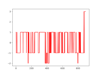
In the tick imbalance bar, the variable we monitor (red) can be positive or negative. It increases/decreases by 1 every time, there is a consecutive increase/decrease in price between ticks. So areas with a steep slope, are areas where there has been a run (one directional movement), which would suggest that the price would have changed relatively more, and hence there is a need for increased sampling. 

In both these algorithms, you will effectively sample more, when the slope of the variable you are tracking is steeper. If the slope is shallower, then that means that the ticks are in line with chance, and the price is likely moving sideways, and hence sample at a slower/normal rate. 

Both algorithms are self-resetting because if an instrument in inherently less noisy or more noisy, the guardrails can be set accordingly. If the base behavior of the instrument changes, in sample, then the algorithms re-sets the guardrails so that we are not over/under sampling

Python Code:

Are there any coding tips to improve speed/execution of the algorithm? Let me know in the comments.....

Code for generating run bars

# Import libraries
import numpy as np
import pandas as pd
import matplotlib.pyplot as plt

# Import dataset
df = pd.read_csv(r'C:\Users\josde\OneDrive\Denny\Deep-learning\Data-sets\Trade-data\ES_Trades.csv')
df = df.iloc[:,0:5]
df['Dollar'] = df['Price']*df['Volume']

# Price change
a = np.diff(df['Price'])
a = np.insert(a,0,0)
df['Delta'] = pd.DataFrame(a)

# Labeling
def labeler(df):
    label = np.ones(len(df['Delta']))
    for i, delta in enumerate(df['Delta']):
        if i > 0:
            if delta == 0:
                label[i] = label[i-1]
            else:
                label[i] = abs(delta)/delta
    df['Label'] = pd.DataFrame(label)
    return df

df = labeler(df)
prob = pd.DataFrame(pd.pivot_table(df,values='Price',index='Label',aggfunc='count'))
prob = np.array(prob)
prob_sell = prob[0]/(prob[0]+prob[1])
prob_buy = prob[1]/(prob[0]+prob[1])
#thresh = 6061 * abs((2*prob_buy)-1)
thresh = 3200.0
thresh_v = np.average(df['Volume']) * thresh
thresh_d = np.average(df['Dollar']) * thresh
# Generate bars
def run(df, thresh,thresh_v,thresh_d):
    bartmp,bartmp_v,bartmp_d = [],[],[]
    collector,collector_v,collector_d  = [],[],[]
    volume_vb,volume_vs,dollar_db,dollar_ds = [],[],[],[]
    beta,beta_v,beta_d = 0.0,0.0,0.0
    beta_b,beta_vb,beta_db = 0.0,0.0,0.0
    beta_s,beta_vs,beta_ds = 0.0,0.0,0.0
    buy,sell,buy_v, sell_v,buy_d, sell_d = 0,0,0,0,0,0
    thresh_tmp,thresh_tmp_v,thresh_tmp_d,study, probe,study_v,probe_v,study_d,probe_d = [],[],[], [], [],[],[],[],[]

    for i, (label,price, volume, dollar) in enumerate(zip(df['Label'],df['Price'],df['Volume'],df['Dollar'])):
        collector.append(price)
        collector_v.append(price)
        collector_d.append(price)



        if label == 1:
            buy = buy + 1
            buy_v = buy_v + 1
            buy_d = buy_d + 1
            beta_b = beta_b + label
            beta_vb = beta_vb + (label*volume)
            beta_db = beta_db + (label*dollar)
            volume_vb.append(volume)
            dollar_db.append(dollar)

        else:
            sell = sell + 1
            sell_v = sell_v + 1
            sell_d = sell_d + 1
            beta_s = beta_s + label
            beta_vs = beta_vs + (label*volume)
            beta_ds = beta_ds + (label*dollar)
            volume_vs.append(volume)
            dollar_ds.append(dollar)

        beta = max(beta_b,abs(beta_s))
        beta_v = max(beta_vb,abs(beta_vs))
        beta_d = max(beta_db,abs(beta_ds))

        if beta >= thresh:
            p_b = buy / (buy+sell)
            p_s = sell / (buy+sell)
            a = len(collector) * max(p_b,p_s)
            thresh_tmp.append(a)
            study.append((p_b,p_s,len(collector),a))
            thresh = np.average(thresh_tmp)
            o = collector[0]
            h = np.max(collector)
            l = np.min(collector)
            c = collector[-1]
            bartmp.append((i,o,h,l,c))
            beta, beta_b, beta_s = 0.0,0.0,0.0
            buy,sell = 0,0
            collector = []

        if beta_v >= thresh_v:
            p_b_v = buy_v / (buy_v+sell_v)
            p_s_v = sell_v / (buy_v+sell_v)
            a = len(collector_v) * max(p_b_v*np.average(volume_vb),p_s_v*np.average(volume_vs))
            thresh_tmp_v.append(a)
            study_v.append((p_b_v,p_s_v,len(collector_v),np.average(volume_vb),np.average(volume_vs),a))
            thresh_v = np.average(thresh_tmp_v)
            o = collector_v[0]
            h = np.max(collector_v)
            l = np.min(collector_v)
            c = collector_v[-1]
            bartmp_v.append((i,o,h,l,c))
            beta_v, beta_vb, beta_vs = 0.0,0.0,0.0
            buy_v,sell_v = 0,0
            collector_v = []
            volume_vb = []
            volume_vs = []

        if beta_d >= thresh_d:
            p_b_d = buy_d / (buy_d+sell_d)
            p_s_d = sell_d / (buy_d+sell_d)
            a = len(collector_d) * max(p_b_d*np.average(dollar_db),p_s_d*np.average(dollar_ds))
            thresh_tmp_d.append(a)
            study_d.append((p_b_d,p_s_d,len(collector_d),np.average(dollar_db),np.average(dollar_ds),a))
            thresh_d = np.average(thresh_tmp_d)
            o = collector_d[0]
            h = np.max(collector_d)
            l = np.min(collector_d)
            c = collector_d[-1]
            bartmp_d.append((i,o,h,l,c))
            beta_d, beta_db, beta_ds = 0.0,0.0,0.0
            buy_d,sell_d = 0,0
            collector_d = []
            dollar_db = []
            dollar_ds = []

    cols = ['Index','Open','High','Low','Close']
    tick_run_bar = pd.DataFrame(bartmp,columns = cols)
    volume_run_bar = pd.DataFrame(bartmp_v,columns = cols)
    dollar_run_bar = pd.DataFrame(bartmp_d,columns = cols)

    cols1 = ['Buy','Sell','Length','Threshold']
    cols1_v = ['Buy','Sell','Length','Buy_vol','Sell_vol','Threshold']
    cols1_d = ['Buy','Sell','Length','Buy_dol','Sell_dol','Threshold']
    study = pd.DataFrame(study,columns = cols1)
    study_v = pd.DataFrame(study_v,columns = cols1_v)
    study_d = pd.DataFrame(study_d,columns = cols1_d)
    return tick_run_bar, volume_run_bar,dollar_run_bar,thresh_tmp, study,study_v,study_d,probe

tick_run_bar, volume_run_bar,dollar_run_bar,thresh_tmp, study,study_v,study_d,probe = run(df, thresh,thresh_v,thresh_d)
print(tick_run_bar.columns, tick_run_bar.shape)
print(study.describe())
print(volume_run_bar.columns, volume_run_bar.shape)
print(study_v.describe())
print(dollar_run_bar.columns, dollar_run_bar.shape)
print(study_d.describe())


# Plot the results
plt.figure(1)
plt.plot(df['Price'], 'r')
plt.figure(2)
plt.plot(tick_run_bar['Open'], 'g')
plt.figure(3)
plt.plot(volume_run_bar['Open'], 'b')
plt.figure(4)
plt.plot(dollar_run_bar['Open'], 'y')
plt.show()

Code for generating imbalance bars

# Import libraries
import numpy as np
import pandas as pd
import matplotlib.pyplot as plt

# Import dataset
df = pd.read_csv(r'C:\Users\josde\OneDrive\Denny\Deep-learning\Data-sets\Trade-data\ES_Trades.csv')
df = df.iloc[:,0:5]
df['Dollar'] = df['Price']*df['Volume']

# Price change
a = np.diff(df['Price'])
a = np.insert(a,0,0)
df['Delta'] = pd.DataFrame(a)

# Labeling
def labeler(df):
    label = np.ones(len(df['Delta']))
    for i, delta in enumerate(df['Delta']):
        if i > 0:
            if delta == 0:
                label[i] = label[i-1]
            else:
                label[i] = abs(delta)/delta
    df['Label'] = pd.DataFrame(label)
    return df

df = labeler(df)
prob = pd.DataFrame(pd.pivot_table(df,values='Price',index='Label',aggfunc='count'))
prob = np.array(prob)
prob_sell = prob[0]/(prob[0]+prob[1])
prob_buy = prob[1]/(prob[0]+prob[1])
#thresh = 6061 * abs((2*prob_buy)-1)
thresh = 800
thresh_v = thresh *np.average(df['Volume'])
thresh_d = thresh *np.average(df['Dollar'])

# Generate bars
def imbalance(df,thresh,thresh_v,thresh_d):
    bartmp,bartmp_v,bartmp_d = [],[],[]
    collector,collector_v,collector_d = [],[],[]
    volume_b,volume_s,dollar_b,dollar_s=[],[],[],[]
    beta, beta_v,beta_d = 0,0,0
    buy,buy_v,buy_d, sell,sell_v,sell_d = 0,0,0,0,0,0
    thresh_tmp, thresh_tmp_v, thresh_tmp_d,study, study_d,study_v = [], [],[],[],[],[]

    for i, (label,price,volume,dollar) in enumerate(zip(df['Label'],df['Price'],df['Volume'],df['Dollar'])):
        collector.append(price)
        collector_v.append(price)
        collector_d.append(price)

        beta = beta + label
        beta_v = beta_v + (label*volume)
        beta_d = beta_d + (label*dollar)

        if label == 1:
            buy = buy + 1
            buy_v = buy_v + 1
            buy_d = buy_d + 1
            volume_b.append(volume)
            dollar_b.append(dollar)

        else:
            sell = sell + 1
            sell_v = sell_v + 1
            sell_d = sell_d + 1
            volume_s.append(volume)
            dollar_s.append(dollar)

        if abs(beta) >= thresh:
            p_b = buy / (buy+sell)
            p_s = sell / (buy+sell)
            a = len(collector) * abs((2 * p_b) - 1)
            thresh_tmp.append(a)
            study.append((p_b,p_s,len(collector),a))
            thresh = np.average(thresh_tmp)
            o = collector[0]
            h = np.max(collector)
            l = np.min(collector)
            c = collector[-1]
            bartmp.append((i,o,h,l,c))
            beta = 0
            buy,sell = 0,0
            collector = []

        if abs(beta_v) >= thresh_v:
            p_b_v = buy_v / (buy_v+sell_v)
            p_s_v = sell_v / (buy_v+sell_v)
            vplus = p_b_v*np.average(volume_b)
            vminus = p_s_v*np.average(volume_s)

            a = len(collector_v) * abs((2 * (vplus)) - (vplus+vminus))
            thresh_tmp_v.append(a)
            study_v.append((p_b_v,p_s_v,len(collector_v),a))
            thresh_v = np.average(thresh_tmp_v)
            o = collector_v[0]
            h = np.max(collector_v)
            l = np.min(collector_v)
            c = collector_v[-1]
            bartmp_v.append((i,o,h,l,c))
            beta_v = 0
            buy_v,sell_v = 0,0
            volume_b,volume_s = [],[]
            collector_v = []

        if abs(beta_d) >= thresh_d:
            p_b_d = buy_d / (buy_d+sell_d)
            p_s_d = sell_d / (buy_d+sell_d)
            vplus = p_b_d*np.average(dollar_b)
            vminus = p_s_d*np.average(dollar_s)

            a = len(collector_d) * abs((2 * (vplus)) - (vplus+vminus))
            thresh_tmp_d.append(a)
            study_d.append((p_b_d,p_s_d,len(collector_d),a))
            thresh_d = np.average(thresh_tmp_d)
            o = collector_d[0]
            h = np.max(collector_d)
            l = np.min(collector_d)
            c = collector_d[-1]
            bartmp_d.append((i,o,h,l,c))
            beta_d = 0
            buy_d,sell_d = 0,0
            dollar_b, dollar_s = [],[]
            collector_d = []

    cols = ['Index','Open','High','Low','Close']
    tick_imbalance_bar = pd.DataFrame(bartmp,columns = cols)
    volume_imbalance_bar = pd.DataFrame(bartmp_v,columns = cols)
    dollar_imbalance_bar = pd.DataFrame(bartmp_d,columns = cols)
    cols1 = ['Buy','Sell','Length','Threshold']
    study = pd.DataFrame(study,columns = cols1)
    study_v = pd.DataFrame(study_v,columns = cols1)
    study_d = pd.DataFrame(study_d,columns = cols1)
    return tick_imbalance_bar, thresh_tmp, study, volume_imbalance_bar,study_v,dollar_imbalance_bar,study_d

tick_imbalance_bar, thresh_tmp, study,volume_imbalance_bar,study_v,dollar_imbalance_bar,study_d  = imbalance(df,thresh,thresh_v,thresh_d)

print(tick_imbalance_bar.columns, tick_imbalance_bar.shape)
print(study.describe())

print(volume_imbalance_bar.columns, volume_imbalance_bar.shape)
print(study_v.describe())

print(dollar_imbalance_bar.columns, dollar_imbalance_bar.shape)
print(study_d.describe())

# Plot the results
plt.figure(1)
plt.plot(df['Price'], 'r')
plt.figure(2)
plt.plot(tick_imbalance_bar['Open'],'g')
plt.figure(3)
plt.plot(volume_imbalance_bar['Open'],'b')
plt.figure(4)
plt.plot(dollar_imbalance_bar['Open'],'y')
plt.show()

#For intuition behind run bars and imbalance bars

# Import Libraries
import pandas as pd
import numpy as np
import matplotlib.pyplot as plt

# Import Data
df = pd.read_csv(r'C:\Users\Denny Joseph\OneDrive\Denny\Deep-learning\Data-sets\Trade-data\ES_Trades.csv')
df = df.iloc[:,0:5]

# Add attributes to the dataframe
df['Dollar'] = df['Volume'] * df['Price']
df['Datetime'] = pd.to_datetime(df['Date'] + " " + df['Time'])
a = np.diff(df['Price'])
a = np.insert(a,0,0)
df['Delta'] = pd.DataFrame(a)
def ticklabeler(df):
    label = np.zeros(len(df['Price']))
    label[0] = 1
    for i, delta in enumerate(df['Delta']):
        if i > 0:
            if delta !=0:
                label[i] = delta/abs(delta)
            if delta == 0:
                label[i] = label[i-1]
    df['Label'] = pd.DataFrame(label)
    return df

df = ticklabeler(df)

def imbalancebar(df):
    cumm = np.zeros(len(df['Price']))
    s = 0
    for i, label in enumerate(df['Label']):
        if i > 500:
            s = s + label
            cumm[i] = s
    df['Imbalance'] = pd.DataFrame(cumm)
    return df

def runbar(df):
    runner = np.zeros(len(df['Label']))
    buy = 0.0
    sell = 0.0
    for i, label in enumerate(df['Label']):
        if i > 500:
            if label == 1.0:
                buy = buy + label

            if label == -1.0:
                sell = (sell + label)

            runner[i] = max(buy,abs(sell))
    df['Run'] = pd.DataFrame(runner)
    return df

df = imbalancebar(df)
df = runbar(df)
print(df.columns)

## Plot
# Primary y axis
fig, ax1 = plt.subplots()
ax1.plot(df.iloc[500:5000,9],'r')
# Secondary y axis
ax2 = ax1.twinx()
ax2.plot(df.iloc[500:5000,10],'g')
plt.show()