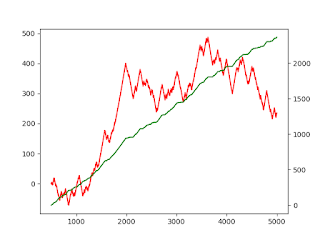
This post will describe how to process & store High Frequency financial data to support your Machine Learning Algorithm, based on how much information is contained in the data The post is directly based on content from the book "Advances in Financial Machine Learning" from Marcos Lopez de Prado Physical meaning: This approach is inspired by Claude Shannon's Information Theory, that is the basis of most compression algorithms. Shannon argued that only departure from the norm is new information. A famous example, is that the sun has risen in the morning. Yes, the event has happened, but because the probability of this event was 1.0, this event does not represent information. In information driven bars, we attempt to use the same insight, to compress the financial data. Here, we know that financial data is inherently noisy, and put guardrails around what level of variance we expect for a particular behavior. It is only when the variance exceeds these guardrails, that we ...
This post will describe some hacks to improve your productivity on Machine Learning projects. This post is scoped around Python development in the PyCharm IDE. Scientific Mode: This feature is only available on the Professional Version of PyCharm. Code blocks: Using # %% at the start of a code block, creates a cell, similar to a cell in Jupyter. You will then have access to a dedicated play button for that cell, allowing you to prototype commands quickly without having to run the entire code block. This adds value when you have a load function in your code, which will take up time to run View variable: You are able to view a sample of the data you have just loaded, and are able to see a plot of that data. This feature is useful during the data exploration stage, as you are trying to build hypothesis. In-line visualisation: You can see the results of cell commands such as seaborn or matplotlib, in line, just by running a cell. Not having to run the entire program, leading to ...
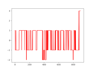
This post will describe how to label a financial dataset to support supervised learning The post is directly based on content from the book "Advances in Financial Machine Learning" from Marcos Lopez de Prado Physical meaning: Algorithm description: Python code: # Import libraries import numpy as np import pandas as pd import matplotlib.pyplot as plt import math # Import data df = pd.read_csv( r'C:\Users\josde\OneDrive\Denny\Deep-learning\Data-sets\Trade-data\ES_Trades.csv' ) df = df.iloc[: , 0 : 5 ] df[ 'Dollar' ] = df[ 'Price' ] * df[ 'Volume' ] print (df.columns) # Generate thresholds d = pd.DataFrame(pd.pivot_table(df , values = 'Dollar' , aggfunc = 'sum' , index = 'Date' )) DOLLAR_THRESHOLD = ( 1 / 50 ) * np.average(d[ 'Dollar' ]) # Generate bars def bar_gen (df , DOLLAR_THRESHOLD): collector , dollarbar_tmp = [] , [] dollar_cusum = 0 for i , (price , dollar) in enumerate ( zip (df[ 'Price...
Comments
Post a Comment