Normalised Mutual information replaces Correlation
The objective of this post is to introduce normalised Mutual Information as a better metric of co-dependency between two variables
Physical meaning: Correlation is a good measure of co-dependency as it is bounded between [0 to 1], and is simple to understand. However, it suffers from a drawback in that it only measures the linear relationship between two variables. If the relationship between two variables is non-linear, as is frequently the case in financial data, we will have low values of correlation, though the variables maybe perfectly predictable using a non-linear function.
Normalised Mutual information is a standardised measure that overcomes these drawbacks. It is based on Information Theory, as opposed to correlation [Linear Algebra], and can accurately quantify the extent to which a relationship exists between two variables [Linear or Non-Linear]. We can then use ML techniques to model the relationship
Experimental results: Using Python code below
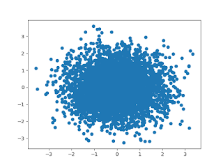
1. Zero Linear Relationship
Value of Correlation Coefficient obtained: 0.00023238753770240598
Value of normalised Mutual Information obtained: 0.005221150748814422
2. Perfect Linear Relationship:
Value of Correlation Coefficient obtained: 0.9999508615918137
Value of normalised Mutual Information obtained: 0.9476343636611047
In the code below, you will see that though the relationship appears normal, we have added a random noise component into the relationship. The Correlation coefficient does not seem to pick this up given the high correlation coefficient. However, the mutual information metric is more sensitive to this, and discounts accordingly.
3. Non Linear Relationship:
Value of Correlation Coefficient obtained: 0.0159978574434585
Value of normalised Mutual Information obtained: 0.5406030932541388
The chart shows that the relationship is non-linear but predictable. The Correlation coefficient does not pick this up as the relationship is not linear, and says there is no relationship. If we use this metric as our guide, we will fail to pick up an opportunity for modeling a relationship. The mutual information recognises a form of relationship and accordingly assigns a higher value of 0.5. This is understandable, as an examination of the chart, will reveal that there are only two possible values of x for every value of y.
Python code:
File: Normalised-Mutual-Information.py# Import Libraries
import numpy as np
import scipy.stats as ss
from sklearn.metrics import mutual_info_score
import matplotlib.pyplot as plt
# Generate data
seed, samples = 0, 5000
x = np.random.normal(size = samples)
e = np.random.normal(size=samples)
# Define the relationship
y = (100 * np.abs(x)) + e
# Calculate the Correlation Coefficient
corr = np.corrcoef(x,y) [0,1]
# Calculate the normalised Mutual Information
hX = ss.entropy(np.histogram(x)[0])
hY = ss.entropy(np.histogram(y)[0])
cXY = np.histogram2d(x,y) [0]
iXY = mutual_info_score(None, None,contingency=cXY)
iXYn = iXY/min(hX,hY)
print(corr,iXYn)
# Plot the data
plt.scatter(x,y)
plt.show()


Comments
Post a Comment